Markov Decision Process
This article is my notes for 16th lecture in Machine Learning by Andrew Ng on Markov Decision Process (MDP). MDP is a typical way in machine learning to formulate reinforcement learning, whose tasks roughly speaking are to train agents to take actions in order to get maximal rewards in some settings. One example of reinforcement learning would be developing a game bot to play Super Mario on its own.
Another simple example is used in the lecture, and I will use it throughout the post as well. Since the example is really simple, so MDP shown below is not of the most general form, but only good enough to solve the example and give the idea of what MDP and reinforcement learning are. The example begins with a 3 by 4 grid as below.
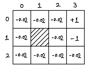
The number in each cell represents the immediate reward when a robot enters it, with discount factor \(\gamma = 0.99\) which will be explained later. The shaded cell represents a place where the robot can not enter. The robot can move in four directions: right, left, up and down. Due to some defects, the robot can only go in the direction it intends with 0.8 probability, and with 0.1 each going into the adjacent directions. For example, if a robot decides to move upward, it will only happen in probability 0.8, and there will be 10% chances going right and 10% chances going left. Moreover, if a robot move in a direction which leads it to leave the grid or into the shaded cell, then it will stay. Finally, we assume that if a robot reaches the cells with +1 or -1, it stops.
Given all these constraints, we want to train a robot, when put at a cell with reward -0.02, to take the best route to the cell with reward 1 and avoid the cell with reward -1.
This is an easy reinforcement learning task, which we will learn how to solve later. Before that, we need to formulate reinforcement learning using MDP, so that we can solve it.
In our example, states can be parametrized by a pair \((i, j)\) indicating the cell at row \(i\) and column \(j\). Thus, we have a set of states
The set of actions \(A\) contains four elements: up(U), down(D), right(R) and left(L), so
We have 11 states and 4 actions, so there are in total 44 state transition distributions. I would only write down two distributions explicitly. The first distribution we want like to look at is taking right at state (1, 2):
The next distribution is to move downward at state \((2, 2)\):
The reward function \(R\) has been already indicated in the figure above. To be more precise, it is
Finally, the discount factor \(\gamma\) is 0.99, which is used in the calculation of payoff. Suppose we have a series of actions applied to initial state \(s_0\), and get the following sequence of states:
The expected payoff of this series of actions at initial state \(s_0\) is defined to be
The goal of reinforcement learning is to choose action for every state so that the expected payoff is maximized.
Let's look at a policy \(\pi\) for our example:
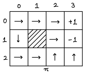
The arrows in the figure represent the actions to take. Note that, states (0, 3) and (1, 3) have no actions since they are places to stop. Now comes a question: How can we calculate \(V^\pi\)? To this end, we need to observe that
This allows us to derived important equations, Bellman equations,
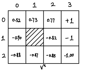
Bellman equations actually give us a system of linear equations which we can use to solve for \(V^\pi(s)\). I am going to implement in python to get \(V^\pi\).
import sys
from collections import defaultdict
py = 'Python ' + '.'.join(map(str, sys.version_info[:3]))
print('Jupyter notebook with kernel: {}'.format(py))

# states and actions
S = [(0, 0), (0, 1), (0, 2), (0, 3), (1, 0), (1, 2),
     (1, 3), (2, 0), (2, 1), (2, 2), (2, 3)]
A = {'U': (-1, 0), 'D': (1, 0), 'R': (0, 1), 'L': (0, -1)}

# reward function
R = {s: -0.02 for s in S}
R[(0, 3)] = 1.0
R[(1, 3)] = -1.0

# transition distributions
P = defaultdict(int)
def helper(s, a):
    h = [(A[a], 0.8)]
    if a in 'UD':
        h.append((A['R'], 0.1))
        h.append((A['L'], 0.1))
    else:
        h.append((A['U'], 0.1))
        h.append((A['D'], 0.1))
    for d, x in h:
        n = s[0]+d[0], s[1]+d[1]
        if n not in S:
            n = s
        yield n, x

for s in S:
    if s in [(0, 3), (1, 3)]:
        continue
    for a in A:
        for n, x in helper(s, a):
            P[s, a, n] += x


# discount factor
gamma = 0.99
Jupyter notebook with kernel: Python 3.6.4
# policy pi
pi = {(0, 0): 'R', (0, 1): 'R', (0, 2): 'R', (0, 3): '#',
      (1, 0): 'D', (1, 1): '#', (1, 2): 'R', (1, 3): '#',
      (2, 0): 'R', (2, 1): 'R', (2, 2): 'U', (2, 3): 'U'}

# calculate value function for pi
# with tolerent error
def val_fn(pi, error=10**(-3)):
    V = {s: 0.0 for s in S}

    while True:
        nV = {}
        for s in S:
            nV[s] = R[s] + gamma * sum(P[s, pi[s], n]*V[n] for n in S)
        epsilon = sum(abs(V[s]-nV[s]) for s in S)
        V = nV
        if epsilon < error:
            break
    return V

V = val_fn(pi)
for s in S:
    print('{}: {:.2f}'.format(s, V[s]))
(0, 0): 0.52
(0, 1): 0.73
(0, 2): 0.77
(0, 3): 1.00
(1, 0): -0.90
(1, 2): -0.82
(1, 3): -1.00
(2, 0): -0.88
(2, 1): -0.87
(2, 2): -0.85
(2, 3): -1.00
Therefore, we get the value function \(V^\pi\) for the policy \(\pi\):
The policy \(\pi\) is far from optimal. In order to find the optimal policy, we need two more definitions.
The optimal value function \(V^\ast\) satisfies also Bellman equations
Moreover, \(\pi^\ast\) can be related to \(V^\ast\) by
These two equations provide two ways to find the optimal policy, value iteration and policy iteration.
Value Iteration
The idea of value iteration is to use the Bellman equations \(\eqref{bellman-ast}\) repeatly to determine \(V^\ast\), then use \(\eqref{pi-ast}\) to find \(\pi^\ast\).
# initialize optimal value function
V = {s: 0.0 for s in S}

# tolerent error
error = 10**(-3)

while True:
    nV = {}
    for s in S:
        nV[s] = R[s] + gamma * max(sum(P[s, a, n]*V[n] for n in S) for a in A)
    epsilon = sum(abs(V[s]-nV[s]) for s in S)
    V = nV
    if epsilon < error:
        break

for s in S:
    print('{}: {:.2f}'.format(s, V[s]))
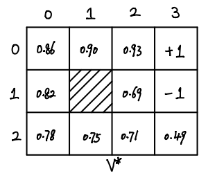
(0, 0): 0.86
(0, 1): 0.90
(0, 2): 0.93
(0, 3): 1.00
(1, 0): 0.82
(1, 2): 0.69
(1, 3): -1.00
(2, 0): 0.78
(2, 1): 0.75
(2, 2): 0.71
(2, 3): 0.49
From the above piece of code, we get \(V^\ast\):
Once we have \(V^\ast\), we can calculate \(\pi^\ast\) easily.
# optimal policy
pi = {s: max(A, key=lambda a: sum(P[s, a, n]*V[n] for n in S))
     for s in S}

for s in S:
    if s in [(0, 3), (1, 3)]:
        continue
    print('{}: {}'.format(s, pi[s]))
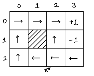
(0, 0): R
(0, 1): R
(0, 2): R
(1, 0): U
(1, 2): U
(2, 0): U
(2, 1): L
(2, 2): L
(2, 3): L
Therefore, \(\pi^\ast\) is
Policy iteration
Policy iteration makes use of equations \(\eqref{pi-ast}\) and \(\eqref{bellman}\). The algorithm goes in this way.
initialize pi randomly
repeat {
  1. calculate value function V for pi
  2. update pi using equation (3)
}
from random import choice

# initialize pi randomly
pi = {s: choice(list(A.keys())) for s in S}

# repeat until stablize
while True:
    V = val_fn(pi)
    npi = {s: max(A, key=lambda a: sum(P[s, a, n]*V[n] for n in S))
          for s in S}
    if pi == npi:
        break
    pi = npi

for s in S:
    if s in [(0, 3), (1, 3)]:
        continue
    print('{}: {}'.format(s, pi[s]))
(0, 0): R
(0, 1): R
(0, 2): R
(1, 0): U
(1, 2): U
(2, 0): U
(2, 1): L
(2, 2): L
(2, 3): L
