Simple Grid Detection for Sudoku
Sudoku is a very interesting puzzle, and it is very easy to get familiar with the rules of the game. I always like to compare sudoku with number theory, they are easy to be understood but can be hard to solve. Fermat's Last Theorem, an easily understood problem even by middle school students, took mathematians 358 years to solve it completely. Solving sudoku puzzles can take even longer: it is proven that solving sudoku puzzels is an NP-complete problem! However, classical 9x9 sudoku puzzles are still feasible using backtracking algorithm. We are not going to talk about how to solve sudoku puzzles here though, we are trying to sovle another problem: detect grids in images containing sudoku puzzles.
To make the problem more concrete, let's make some assumption on the image that contains a sudoku puzzle:
- The image only contains one sudoku puzzle
- The sudoku puzzle is the largest block in the image
- There is no/little distorsion/rotation of the sudoku puzzle grid
Also in this article, we focus on only simple solutions without heavy image processing. We will use Pillow to read images and convert them to gray scale images, and we use Numpy to manipulate images as arrays. For visualization, we use Matplotlib.
import sys
py = 'Python ' + '.'.join(map(str, sys.version_info[:3]))
print('Jupyter notebook with kernel: {}'.format(py))

import time
from PIL import Image
import numpy as np
import matplotlib.pyplot as plt
Jupyter notebook with kernel: Python 3.7.0
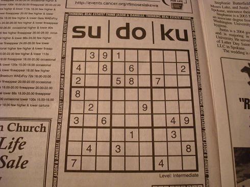
We will first load some images of sudoku puzzles that we are going use througout the article. All images are collected from the internet. I put a copy of these images here: sudoku0.jpg, sudoku1.jpg, sudoku2.jpg
images = []
for n in range(3):
    # read the image
    img = Image.open(f'sudoku/sudoku{n}.jpg')
    # convert image to gray scale
    img = img.convert('L')
    images.append(np.array(img))

plt.figure(figsize=(15, 30))
for n in range(3):
    plt.subplot(1, 3, n+1)
    plt.imshow(images[n], cmap='gray')
    plt.xticks([])
    plt.yticks([])
plt.show()

0. Setup
In this section, we are going to setup some codes for later use. We will create a base class GridDetector: it will assume the middle part of the image is the grid of the sudoku puzzle. We will subclass GridDetector to implement better solutions later. We will also define a function check(DetectorClass, images) to visually show the results of our grid detectors.
class GridDetector:

    def __init__(self, image):
        self.image = image
        self.row, self.col = self.image.shape

        # coords is a tuple (x1, y1, x2, y2) representing the bounding
        # box of the detected grid
        self.coords = None

    def grid(self):
        '''Return a tuple (x1, y1, x2, y2) indicating the grid,
        where (x1, y1) is the upper left corner of the grid,
        and (x2, y2) is the lower right corner of the grid.

        All subclass should implement this method.'''
        if self.coords is not None:
            return self.coords
        x1 = int(self.col * 0.15)
        y1 = int(self.row * 0.15)
        x2 = int(self.col * 0.85)
        y2 = int(self.row * 0.85)
        self.coords = (x1, y1, x2, y2)
        return (x1, y1, x2, y2)

    def plot(self, plt):
        plt.imshow(self.image, cmap='gray')
        start = time.time()
        x1, y1, x2, y2 = self.grid()
        time_used = time.time() - start
        plt.plot([x1, x1], [y1, y2], 'r-', lw=5)
        plt.plot([x1, x2], [y2, y2], 'r-', lw=5)
        plt.plot([x2, x2], [y1, y2], 'r-', lw=5)
        plt.plot([x1, x2], [y1, y1], 'r-', lw=5)
        plt.xticks([])
        plt.yticks([])
        plt.title(f'Detection Time: {time_used:.2}s')

def check(DetectorClass, images):
    n = len(images)
    plt.figure(figsize=(15, 30))
    for i, image in enumerate(images):
        plt.subplot(1, n, i+1)
        DetectorClass(image).plot(plt)
    plt.show()

check(GridDetector, images)

1. Largest Black Connected Component
Our first idea makes use of the second assumption on the image: the sudoku puzzle is the largest block in the image. Recall that in a gray scale image, a pixel of value 0 is black and that of value 255 is white. However, the pixels forming the grid do not have to be of value 0 to look black. Indeed, we will treat pixels with value less than 80 black. We then use flood fill algorithm to find the largest black connected component, which we will assume to be the grid we are looking for.
class LargestComponent(GridDetector):

    threshold = 80

    def grid(self):
        if self.coords is not None:
            return self.coords
        visited = set()
        for i in range(self.row):
            for j in range(self.col):
                if (i, j) in visited or self.image.item(i, j) >= self.threshold:
                    continue
                x1, y1, x2, y2 = self._flood_fill(i, j, visited)
                if self.coords is None:
                    self.coords = (x1, y1, x2, y2)
                else:
                    a1, b1, a2, b2 = self.coords
                    if (x2 - x1) * (y2 - y1) > (a2 - a1) * (b2 - b1):
                        self.coords = (x1, y1, x2, y2)
        return self.coords

    def _flood_fill(self, i, j, visited):
        r1 = r2 = i
        c1 = c2 = j
        stack = [(i, j)]
        visited.add((i, j))
        while stack:
            r, c = stack.pop()
            for nr, nc in [(r+1, c), (r-1, c), (r, c+1), (r, c-1)]:
                if nr < 0 or nc < 0 or nr >= self.row or nc >= self.col:
                    continue
                if (nr, nc) in visited or self.image.item(nr, nc) >= self.threshold:
                    continue
                r1 = min(nr, r1)
                r2 = max(nr, r2)
                c1 = min(nc, c1)
                c2 = max(nc, c2)
                stack.append((nr, nc))
                visited.add((nr, nc))
        return (c1, r1, c2, r2)

check(LargestComponent, images)

We can see that this method works quite well except for the first image. This is because the first image has black frame wrapping around the whole image and our algorithm detects it as our largest component. An ad hoc solution is to crop the image to remove the black frame.
image0 = images[0][20:-20, 20:-20]
check(LargestComponent, [image0])

We now detect the correct bounding box for the grid. However, it takes several seconds to finish the detection. The algorithm in LargestComponent needs to examinate every pixel and its time complexity is linear to the size of the image. The first image has size 1109 x 1600, which is not that big actually. I guess the problem has something to do with the speed of Python.
2. Low Average of Rows and Columns
We know that black pixels have small values (close to 0) while whit pixels have large values (close to 255) in a gray scale image, so we expect the average value of the row that contains a line to be smaller. We can confirm this with some simple plots.
img = images[0]
row, col = img.shape
plt.figure(figsize=(6, 8))
plt.imshow(img, cmap='gray')
plt.show()
plt.figure(figsize=(12, 4))
plt.subplot(121)
plt.plot(range(row), np.sum(img, axis=1) / col)
plt.title('Row Average')
plt.subplot(122)
plt.plot(range(col), np.sum(img, axis=0) / row)
plt.title('Column Average')
plt.show()


By looking at the graphs above, we see that the valleys of the graphs might indicate the rows or columns of the grid. So we need a way to identify valleys in the graphs.
def valleys(vals, dist=20, num=20):
    '''Identify first `num` valleys in the array `vals`, with
    the assumption that two valleys are at least `dist` away
    from each other.'''
    candidates = []
    for i, v in enumerate(vals):
        if i == 0 or i == len(vals) - 1:
            continue
        if vals[i + 1] > v and vals[i - 1] > v:
            candidates.append((i, v))
    candidates.sort(key=lambda x: x[1])
    ans = []
    for i, v in candidates:
        if any(abs(i - j) < dist for j, _ in ans):
            continue
        ans.append((i, v))
        if len(ans) == num:
            break
    return [a[0] for a in ans], [a[1] for a in ans]

def show_valleys(img):

    row, col = img.shape

    plt.figure(figsize=(12, 4))

    # plot figure: Row Average valleys
    plt.subplot(121)
    row_vals = np.sum(img, axis=1) / col
    rows, vals = valleys(row_vals, num=10)
    plt.plot(range(row), row_vals)
    plt.scatter(rows, vals, color='red')
    plt.title('Row Average')

    # plot figure: Column Average with valleys
    plt.subplot(122)
    col_vals = np.sum(img, axis=0) / row
    cols, vals = valleys(col_vals, num=10)
    plt.plot(range(col), col_vals)
    plt.scatter(cols, vals, color='red')
    plt.title('Column Average')
    plt.show()

show_valleys(images[0])

In each graph above, we identify the first 10 valleys (the red dots) that at least 20 pixels away from other valleys. We can use these valleys to help determine the position of the grid. With some confidence, we assume that these 10 valleys mostly correspond to 10 lines of the grid. We try to identify 10 lines of a grid from an array of values. Thus finding a 9x9 grid in a 2-dimensional image now becomes a problem of finding a grid of valleys in a 1-dimensional array.
Suppose we are given an array vals of values and we would like to find a grid of valleys. By a voting process, we can determine the spacing of the grid. For example, in the Row Average figure above, the 4th, 5th, 6th, 7th and 8th valleys roughly have the same spacing to its neighbor. We will assume that spacing is the spacing in the grid. Suppose the spacing we get is \(d\), then to determine the grid, we just need to find first index of the grid.
Since we know the spacing \(d\) of the grid, if we know first index \(i\) of the grid, we can compute all coordinates of the grid: \(i, i+d, \dots, i+9d\). We would like all these indices corresponds to valleys. Therefore, we might use the following formula to determine \(i\):
where \(i\) runs over all possible index of the first row.
class LowAverage(GridDetector):

    def grid(self):
        if self.coords is not None:
            return self.coords

        row_vals = np.sum(self.image, axis=1) / self.col
        col_vals = np.sum(self.image, axis=0) / self.row

        row_index, row_spacing = self._grid1D(row_vals)
        col_index, col_spacing = self._grid1D(col_vals)

        x1, x2 = col_index, col_index + col_spacing * 9
        y1, y2 = row_index, row_index + row_spacing * 9
        self.coords = (x1, y1, x2, y2)

        return self.coords

    def _grid1D(self, vals):
        idx, _ = valleys(vals, num=10)
        idx.sort()
        sp = list(sorted(b - a for a, b in zip(idx[:-1], idx[1:])))

        threshold = 10
        sp.append(sp[-1] + threshold * 2)
        votes = 0
        spacing = 0
        tmp = []
        for s in sp:
            if not tmp:
                tmp.append(s)
                continue
            if s - tmp[-1] <= threshold:
                tmp.append(s)
            else:
                if votes < len(tmp):
                    votes = len(tmp)
                    spacing = int(sum(tmp) / votes)
                tmp = [s]
        weights = 2 ** 32
        index = 0
        for i in range(len(vals) - spacing * 9):
            w = sum(vals[i+spacing*j] for j in range(10))
            if w < weights:
                index = i
                weights = w
        return index, spacing


check(LowAverage, images)

The algorithm works well to find the correct spacing for all three images. And it correctly ignores the black frame of the first image. Moreover, it takes much less time to detect the grid than that of LargestComponent. The time complexity of this algorithm is the same as the one from LargestComponent. It runs faster because it uses Numpy operations. From the second image, we know that the algorithm is very sensitive to distorsion of images.
3. The End
These two simple solutions works well for nice and clean images like the third image above. In general, both of them will fail. The accuracy of the solutions can be improved by some image pre-processing with OpenCV. For example, we can remove noises, reduce distortion and etc. We shall see in a later article how we can use OpenCV to detect grids with higher accuracy.
