Introduction

在这篇文章中，我将使用朴素贝叶斯分类器(Naive Bayes Classifier)打造一个简单的个人推荐系统：给定一篇中文文章(article)，返回我喜欢(like)这篇文章的概率。用数学的语言来描述的话，我们要计算的是

根据贝叶斯公式，

我一直想把自己的微信聊天记录导出来，用来做一些奇奇怪怪的东西。可以用来分析一下过去一年里跟谁聊天了，聊的都是啥，或者做一个带有自己特点的聊天机器人。问题是，微信现在并没有简单导出聊天记录的方法。从我网上搜到的资料，安卓机器上的微信会将聊天记录（还有很多其他数据，比如联系人）保存在一个叫做EnMicroMsg.db的数据库中。这个数据库是使用SQLCipher生成的，没有密码是无法正常打开的。这个密码其实可以很容易通过自己手机的信息以及微信的信息计算出来，我也根据网上的教程计算出属于我的密码了。但是我一直没有成功解密我的聊天记录数据库。直到今天我再次搜寻了关于微信数据库的资料，才发现我不仅仅需要密码，还需要其他一下数据库的设置才能正确打开。这篇博文主要的目的是记录我该怎么做才能导出微信聊天记录，以方便以后使用。

昨天跟永佳在路村看了音乐剧《悲惨世界》，演员细腻的表演与出色舞台灯光效果让我对舞台剧的热爱更深一分。

最近看了一些关于卷积网络（Convolution Neural Network）的内容，我想用mnist数据集重复一下网上的教程，好让自己能更好地理解并使用卷积网络。比较了一下Tensorflow和Pytorch，个人比较喜欢Pytorch，所以以后基本就用它了。Pytorch里是包含获取mnist数据集的api的，使用这api我们可以很简单就能准备好数据。但是出于学习Pytorch的目的，我决定自己准备数据。

之前我在另一篇博文用了广义线性模型Softmax来识别这些手写数字，错误率最低达到了7.77%。使用图像识别领域上常用有效的卷积网络，我们会得到更低的错误率。这点会在本文后面看到。这篇博文不会用太多的文字解释，基本上都是代码。

好久没有比赛了，上次比赛还是去年11月了。这次比赛表现比较差，只做出了前两道。后来发现，第三道我跟小伙伴都有正确的想法了，只是没有意识到答案允许有10^-6的误差。

第一题Subdomain Visit Count

比较简单的统计。

class Solution:
    def subdomainVisits(self, cpdomains):
        """
        :type cpdomains: List[str]
        :rtype: List[str]
        """
        cnt = collections.defaultdict(int)
        for cp in cpdomains:
            n, addr = cp.split(' ')
            n, addr, p = int(n), '.'+addr, 0
            while p != -1:
                addr = addr[p+1:]
                cnt[addr] += n
                p = addr.find('.')
        return ['{} {}'.format(v, k) for k, v in cnt.items()]

This post is considered to the notes on finite horizon Markov decision process for lecture 18 in Andrew Ng's lecture series. In my previous two notes ([1], [2]) about Markov decision process (MDP), only state rewards are considered. We can easily generalize MDP to state-action reward.

State-Action Reward

Our reward function now is a function in terms of both states and actions. More precisely, the reward function is a function

All other requirements in definition of MDP will remain intact. For completeness, we include the definition here. We shall pay attention to the fifth components.

I wrote this post for lecture 17 in Andrew Ng's lecture collections on Machine Learning. In my previous post, we discussed Markov Decision Process (MDP) in its simplest form, where the set of states and the set of actions are both finite. But in real world application, states and actions can be infinite and even continuous. For example, if we want to model states of a self-driving car in a 2D plane, we must at least have the position \((x, y)\), the direction \(\theta\) of the car pointing to, its velocity \((v_x, v_y)\) and the rate \(r\) of change in \(\theta\). So the states of a car is at least a 6 dimensional space. For actions of a car, we can control how fast it goes in direction \(\theta\) and we can also control \(r\). Thus the actions have dimension 2.

In this post, we consider only continuous states with finite actions. Indeed, actions space usually has much lower dimension than states space, so in case of continuous actions, we might just discretize the actions spaces to get a finite set of representatives of actions. One may argue that we can also discretize the states space. Yes, we can do it, but only when the dimension \(n\) of state space is small enough: if we discretize each dimension into \(k\) parts, then there would be \(k^n\) many states. If \(n\) is large, then \(k^n\) is not feasible. This is so called the curse of dimensionality. Moreover, discretizing states space usually results in lack of smoothness.

This article is my notes for 16th lecture in Machine Learning by Andrew Ng on Markov Decision Process (MDP). MDP is a typical way in machine learning to formulate reinforcement learning, whose tasks roughly speaking are to train agents to take actions in order to get maximal rewards in some settings. One example of reinforcement learning would be developing a game bot to play Super Mario on its own.

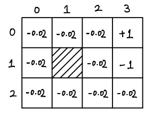
Another simple example is used in the lecture, and I will use it throughout the post as well. Since the example is really simple, so MDP shown below is not of the most general form, but only good enough to solve the example and give the idea of what MDP and reinforcement learning are. The example begins with a 3 by 4 grid as below.

周末晚（14号）我终于去看了久闻的歌剧魅影，果然十分震撼。

This article is my notes on Principal Component Analysis (PCA) for Lecture 14 and 15 of Machine Learning by Andrew Ng. Given a set of high dimensional data \(\{x^{(1)}, \dots, x^{(m)}\}\), where each \(x^{(i)} \in \R^{n}\), with the assumption that these data actually roughly lie in a much smaller \(k\) dimensional subspace, PCA tries to find a basis for this \(k\) dimensional subspace. Let's look at a simple example: